Titin exon specific GERP scores

Coming back to Titin gene, are all exons equally important? GERP scores could tell us something about how the exons vary in conservation level at base-pair resolution.

In the above figure, the y-axis is the exon rank and the x-axis has boxplots of GERP scores for each exon. Exons with mean GERP scores above 0 are colored red and those below zero are colored blue. One can clearly see the GERP score reduce considerably between exons 160 and 200.

HGT candidate genes - GERP score distribution

HGT candidate genes have been identified in vertebrate species based on gene absence/presence in metazoans. The actual workflow can be found in figure S4.

Interestingly, they identify 145 genes that are candidates for HGT into all primates from various taxon and another 51 from viruses. They provide Ensemble gene id's for these genes in the Human genome.

Of the 145 genes, only 135 could be found in the Ensemble biomart today (Ensemble 79). The following ten genes have been "retired" and are not used in below analysis. These genes seem to be randomly drawn from the different "confidence classes" used in the paper.

ENSG00000107618    class A HGT    Validated
ENSG00000157358    class A HGT    Validated
ENSG00000196333    class C HGT    Not-validated
ENSG00000204486    class C HGT    Validated
ENSG00000204502    class C HGT    Validated
ENSG00000204513    class C HGT    Validated
ENSG00000212857    class C HGT    Not-validated
ENSG00000256062    class A HGT    Validated
ENSG00000260383    class B HGT    Not-validated
ENSG00000263074    class B HGT    Validated

ENSG00000107618 has been merged with ENSG00000265203 which is also a HGT candidate. ENSG00000256062 has been merged into ENSG00000175164, this is the much talked about ABO blood group gene. ENSG00000260383 has been merged into ENSG00000179832 which also happens to be a HGT candidate. ENSG00000263074 is merged into ENSG00000141337 (arylsulfatase G).

A total of 4018 exons could be found for these 135 genes. GERP scores could not obtained for 8 of these genes [ENSG00000066813,ENSG00000183248,ENSG00000183549,ENSG00000183747,
ENSG00000204510,ENSG00000229571,ENSG00000232423,ENSG00000243073]. Here, we obtain the GERP scores for each base of all these exons. Example code from the web was updated to use a bed file as input and print the GERP score for each base within the bed intervals.

 #!/usr/bin/env perl  
 use strict;  
 use warnings;  
 use lib '~/biomart-perl/lib';  
 use Bio::EnsEMBL::Registry;  
 use Bio::EnsEMBL::Utils::Exception qw(throw);  
 my $reg = "Bio::EnsEMBL::Registry";  
 my $species = "Homo sapiens";  
 my $line = "";  
 open FILE1, $ARGV[0] or die $!;  
 $reg->load_registry_from_db(  
    -host => "ensembldb.ensembl.org",  
    -user => "anonymous",  
 );  
 #get method_link_species_set adaptor  
 my $mlss_adaptor = $reg->get_adaptor("Multi", "compara", "MethodLinkSpeciesSet");  
 my $mlss = $mlss_adaptor->fetch_by_method_link_type_species_set_name("GERP_CONSERVATION_SCORE", "mammals");  
 throw("Unable to find method_link_species_set") if (!defined($mlss));  
 my $slice_adaptor = $reg->get_adaptor($species, 'core', 'Slice');  
 throw("Registry configuration file has no data for connecting to <$species>") if (!$slice_adaptor);  
 my $cs_adaptor = $reg->get_adaptor("Multi", 'compara', 'ConservationScore');                 
 while($line=<FILE1>){  
 #$line=$ARGV[0];  
 chomp $line;  
 my @parts=split('\t',$line);  
 my $seq_region = $parts[0];  
 my $seq_region_start = $parts[1];  
 my $seq_region_end =  $parts[2];  
 my $slice = $slice_adaptor->fetch_by_region('toplevel', $seq_region, $seq_region_start, $seq_region_end);  
 throw("No Slice can be created with coordinates $seq_region:$seq_region_start-$seq_region_end") if (!$slice);  
 my $display_size = $slice->end - $slice->start + 1;   
 my $scores = $cs_adaptor->fetch_all_by_MethodLinkSpeciesSet_Slice($mlss, $slice, $display_size);  
 #print "number of scores " . @$scores . "\n";  
 foreach my $score (@$scores) {  
   if (defined $score->diff_score) {  
 #     printf("position %d observed %.4f expected %.4f difference %.4f\n", $score->position, $score->observed_score, $score->expected_score, $score->diff_score);  
      printf("$parts[3]\t$parts[4]\t%.4f\n",$score->diff_score);  
   }  
 }  
 }  
 close FILE1;  

Negative GERP scores suggest that the sites are probably evolving neutrally.

 read.table(file="GERP.scores",header=FALSE,stringsAsFactors=FALSE)->M  
 as.data.frame(aggregate(M,list(M$V2),mean))->N  
 as.data.frame(aggregate(M,list(M$V2),max))->P  
 N$Group.1[N$V3<0]->negative.mean.GERP  
 jpeg("GERP_HGT_distribution.jpeg")  
 boxplot(as.numeric(M$V3)~M$V2,outline=FALSE,col=ifelse(unique(M$V2) %in% negative.mean.GERP, "red", "blue"),xaxt="n",ylab="GERP score",main="GERP score by gene")  
 legend("bottomright", c("Negative mean GERP", "Positive mean GERP"), fill = c("red", "blue"))  
 dev.off()  

Despite 41 genes having a mean GERP score less than 0, each of these genes have atleast a few sites that are having positive GERP scores.

Based on above arguments, it could be suggested that 10 of the 145 genes are probably annotation artifacts. The 127 genes for which GERP scores could be obtained from whole genome alignments show moderate levels of conservation, suggesting these genes are probably not artifacts.

Lack of Isolation By Distance pattern in Tiger mitochondrial data

A recent paper, that used ancient DNA sequences from museum samples concluded that Bali, Javan and Sumatran tigers had a closer genetic relationship by comparing it with diagnostic mtDNA sequences from various other tiger subspecies.

Due to lack of precise geographic information about the sampling locations, despite having a matrix of genetic distances they could not look at isolation by distance patterns. The historical geographic ranges of these subspecies can be found on wikipedia. One could, just assume sampling locations within the geographic range and check if a pattern of IBD can be seen. While performing such assumptions in a paper might not be possible, a blog provides you some freedom to do so. However, somebody familiar with Tigers might be able to provide better assumptions. 

ALT or Siberian Tiger is assumed to have been sampled from Sikhote-Alin    45°N 136°E. VIR or Caspian Tiger from Gansu 38°N 102°E. AMO or South China Tiger from Qin mountains 33°N 107°E. COR or Indo-chinese Tiger from Yunnan 25°N 101°E. JAX or Malayan Tiger from Kelantan 5°N 102°E. SUM or Sumatran Tiger from Bukit Barisan Selatan National Park 5°S 104°E. SON or Javan Tiger from Java 7°S 110°E. BAL or Bali Tiger from Bali 8°S 115°E. TIG or Bengal Tiger from Hazaribagh National Park 24°N 85°E.

The R package sp provides many useful functions to deal with spatial data. We use the spDistsN1 function to get the using Euclidean or Great Circle distance between two co-ordinates.

 library(sp)  
 library(reshape)  
 library("ecodist")  
 someCoords <- data.frame(long=c(136,102,107,101,102,104,110,115,85), lat=c(45,38,33,25,5,5,7,8,24))  
 apply(someCoords, 1, function(eachPoint) spDistsN1(as.matrix(someCoords), eachPoint, longlat=TRUE))->X  
 X[upper.tri(X)]->G  
 pop1<-c("ALT","ALT","ALT","ALT","ALT","ALT","ALT","ALT","VIR","VIR","VIR","VIR","VIR","VIR","VIR","AMO","AMO","AMO","AMO","AMO","AMO","COR","COR","COR","COR","COR","JAX","JAX","JAX","JAX","SUM","SUM","SUM","SON","SON","BAL")  
 pop2<-c("VIR","AMO","COR","JAX","SUM","SON","BAL","TIG","AMO","COR","JAX","SUM","SON","BAL","TIG","COR","JAX","SUM","SON","BAL","TIG","JAX","SUM","SON","BAL","TIG","SUM","SON","BAL","TIG","SON","BAL","TIG","BAL","TIG","TIG")  
 data.frame(pop1,pop2,G)->Geodist  
 Geodist2 <- with(Geodist, G)  
 nams <- with(Geodist, unique(c(as.character(pop1), as.character(pop2))))  
 attributes(Geodist2) <- with(Geodist, list(Size = length(nams),Labels = nams,Diag = FALSE,Upper = FALSE,method = "user"))  
 class(Geodist2) <- "dist"  
 read.table(file="Tiger_Fst.txt",header=TRUE,sep="\t",row.names = 1)->M  
 na.omit(melt(M))->N  
 data.frame(pop1,pop2,N$value)->Gendist  
 Gendist2 <- with(Gendist, N$value)  
 nams <- with(Gendist, unique(c(as.character(pop1), as.character(pop2))))  
 attributes(Gendist2) <- with(Gendist, list(Size = length(nams),Labels = nams,Diag = FALSE,Upper = FALSE,method = "user"))  
 class(Gendist2) <- "dist"  
 mantel(Geodist2 ~ Gendist2, nperm=10000)  
   mantelr    pval1    pval2    pval3  llim.2.5% ulim.97.5%   
 -0.06313036 0.67800000 0.32230000 0.65900000 -0.25930292 0.12999925   
 jpeg("Tiger_isolation_by_distance.jpeg")  
 plot(G,N$value/(1-N$value),xlab="Distance in Km",ylab="Fst/(1-Fst) from mtDNA sequences",main="Isolation by Distance pattern",pch=16,col="blue",xlim=c(0,6000))  
 text(G,N$value/(1-N$value),labels=paste(pop1,"  ",pop2))  
 dev.off()  
 jpeg("Tiger_Fst_cladogram.jpeg")  
 hc = hclust(dist(Gendist2))  
 op = par(bg = "#DDE3CA")  
 plot(hc, col = "#487AA1", col.main = "#45ADA8", col.lab = "#7C8071", col.axis = "#F38630", lwd = 3, lty = 3, sub = "", hang = -1, axes = FALSE,xlab="",main="Tiger Fst cladogram")  
 axis(side = 2, at = seq(0, 400, 100), col = "#F38630", labels = FALSE,   lwd = 2)  
 mtext(seq(0, 400, 100), side = 2, at = seq(0, 400, 100), line = 1, col = "#A38630", las = 2)  
 dev.off()  

The mantel's test shows that the IBD pattern has a very weak negative correlation. This is not entirely unexpected, given the high values of Fst that are almost saturated. Would using more markers with greater resolution capture a IBD pattern? How strong are the bottlenecks?

 

They have already used the data to build a phylogenetic tree and a network. As i need to do something different, i build a cladogram using the Fst matrix. While this cladogram shows that the SUM and BAL are close to each other, it fails to group SON with them. Various other differences from the phylogenetic tree can be seen. 

Dog genome annotation quality has improved during the past 30 Ensembl releases

Quality of genome annotation changes with each new Ensembl release. How much does the quality actually change? 

We can quantify the amount of change in annotation quality by looking at specific parameters like number of genes, transcripts, exons etc. Here, the annotation of the dog genome from Ensembl release 48 to 78 is compared to understand the effect of change in genome assembly as well as role of annotation curation. 

First, we see the number of annotated genes(y-axis) in the Dog genome vs the Ensembl release(x-axis). It can be seen that the number of genes steadily  keeps increasing with each release. However, the sharp drop in number of genes in release 68 is surprising. The drop in number of genes from release 67 to 68 is less surprising as that release was accompanied by a change in genome assembly from BROADD2 to CanFam3.1

Various other features of the genome annotation such as Number of transcripts per Gene, Median coding length, Average Exons per gene and 3' UTR count change in a very different way (see below figure)

While such large changes in the genome annotation between releases might be scary, the engine of science chugs on. In the broader scheme of things, the fact that the Dog has 23,062 genes or 24,660 genes should hopefully not matter for the Dog breeders who seem to be driven by the discoveries made possible by the Dog genome and its annotation.

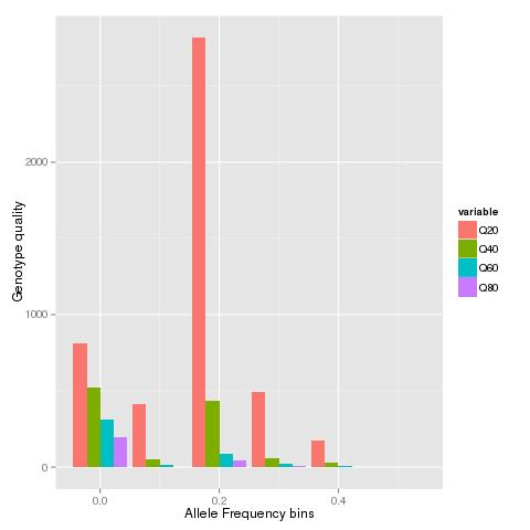
Effect of genotype qaulity on the site frequency spectrum

The below shell script takes vcf file as an argument in the for loop and calculates the allele frequencies using VCFTools. These allele frequencies are used to calculate a folded SFS by taking only the major alleles in the calculation.

 for VCF in vcf_file_name.vcf  
 do  
 mkdir "$VCF".dir  
 cd "$VCF".dir  
 cp ../data/"$VCF" .  
 for GQ in 20 40 60 80  
 do  
 #calculate allele frequencies with VCFtools  
 vcftools --vcf "$VCF" --freq --out test.af --minGQ "$GQ"  
 #Take vcf file and extract columns with allele frequency data, in this case the freq output we want columns five and six  
 cut -f5 test.af.frq > test_col1  
 cut -f6 test.af.frq > test_col2  
 cat test_col1 test_col2 > test_append  
 #removes blank line  
 sed -e '/^ *$/d' test_append > test_append2  
 #get rid of first line and first two characters (a/t/g/c:)  
 sed 1d test_append2 > test_append3  
 cat test_append3 | sed 's/^..//' > FILENAME_AFS  
 #To keep only values below 0.50  
 awk '$NF <0.50' FILENAME_AFS > FILENAME_AFS_50."$GQ"  
 echo "0" >> FILENAME_AFS_50."$GQ"  
 echo "0.1" >> FILENAME_AFS_50."$GQ"  
 echo "0.2" >> FILENAME_AFS_50."$GQ"  
 echo "0.3" >> FILENAME_AFS_50."$GQ"  
 echo "0.4" >> FILENAME_AFS_50."$GQ"  
 echo "0.5" >> FILENAME_AFS_50."$GQ"  
 rm FILENAME_AFS test.af.frq test.af.log test_append test_append2 test_append3 test_col1 test_col2  
 done  
 cp ../makebars.r .  
 Rscript makebars.r  
 cd ..  
 done  

The rscript makebars is used to read in each of the site frequency spectrum's at the different genotype quality thresholds and generate a barplot of the SFS.

 read.table(file="FILENAME_AFS_50.20",header=FALSE)->AF20  
 read.table(file="FILENAME_AFS_50.40",header=FALSE)->AF40  
 read.table(file="FILENAME_AFS_50.60",header=FALSE)->AF60  
 read.table(file="FILENAME_AFS_50.80",header=FALSE)->AF80  
 as.data.frame(table(round(AF20$V1,1)))->A20  
 as.data.frame(table(round(AF40$V1,1)))->A40  
 as.data.frame(table(round(AF60$V1,1)))->A60  
 as.data.frame(table(round(AF80$V1,1)))->A80  
 data.frame(Q20=A20$Freq,Q40=A40$Freq,Q60=A60$Freq,Q80=A80$Freq)->q  
 library(plyr)  
 library(ggplot2)  
 library(reshape)  
 Names=seq(0,0.5,0.1)  
 data=data.frame(cbind(q),Names)  
 data.m <- melt(data, id.vars='Names')  
 cbbPalette <- c("#000000", "#E69F00", "#56B4E9", "#009E73", "#F0E442", "#0072B2", "#D55E00", "#CC79A7")  
 jpeg("barplot.jpeg")  
 ggplot(data.m, aes(Names, value,fill = variable)) + geom_bar(stat="identity",position="dodge")+ xlab("Allele frequency bins") + ylab("Number of sites")  
 dev.off()  

When the VCF file from a published study is run through the script will generate a graph like below:

NOD Mice Substrain Divergence - Runs of Homozygosity

Divergence or rather Differentiation (to use the right terminology), between natural ecotypes or subspecies has been studied in multiple pairs. The broad-scale patterns and underlying processes for such genome wide changes has been studied in detail. 

Do similar processes govern the "divergence" of  artificially inbred strains? Is Drift too strong for background selection to be relevant in such inbred lines? Data [Genetic Analysis of Substrain Divergence in NOD Mice] from a recent study of NOD mice sub-strains might provide some answers. While the study was restricted to sites fixed to homozygosity, it does provide some idea of the major regions that differ between the mouse strains. More detailed analysis of the mouse strains including multiple individuals might be necessary to understand if the diversity landscape of the genome has played any role in shaping the accumulation of genetic differences. 

The Supplementary table 4 provides a list of all the SNP's genotyped using the Mouse Diversity Array. We try to identify runs of homozygosity that share the same genealogy and note if these regions correspond to the deletions identified and validated in the study.

Position				Variants
Chr	Pos (mm10)	Idd.region	SnpId	Type	BomTac	MrkTac	ShiJcl	ShiLtDvs	ShiLt
1	14207005		JAX00242533	G/C	G	G	G	C	C
1	39035554	Idd26	JAX00002691	T/-	T	T	-	T	T
1	39035867	Idd26	JAX00247792	C/-	C	C	-	C	C
1	39035916	Idd26	JAX00002693	A/-	A	A	-	A	A
1	39057575	Idd26	JAX00002694	C/-	C	C	-	C	C
1	111005763	Idd5.4a	JAX00262691	A/-	A	-	A	A	A
1	111014417	Idd5.4a	JAX00262692	T/-	T	-	T	T	T
1	111019979	Idd5.4a	JAX00262694	G/-	G	-	G	G	G
2	83392830		JAX00494876	G/-	-	-	G	-	G
2	131300866	Idd13, Idd13-not B2m	JAX00503778	A/G	A	A	A	G	A
3	8893755		JAX00514596	C/A	C	C	C	C	A
3	24286919		JAX00516977	C/-	C	C	C	-	-
3	24320030		JAX00516979	T/-	T	T	T	-	-
3	24348995		JAX00105316	A/G	A	A	A	-	-
3	24383100		JAX00516985	T/-	T	T	T	-	-
3	33847305		JAX00106024	-/G	G	G	-	G	G
3	33847927		JAX00519037	-/T	T	T	-	T	T
3	33848126		JAX00519038	-/A	A	A	-	A	A
3	33850816		JAX00519044	-/C	C	C	-	C	C
3	33851250		JAX00519045	A/-	A	A	-	A	A
3	33851593		JAX00519046	G/-	G	G	-	G	G
3	65332947		JAX00525208	T/C	T	T	T	T	C
4	44176075		JAX00549396	T/A	T	T	T	A	A
4	95778743		JAX00558533	G/A	G	G	G	A	G
5	22274118		JAX00575925	T/C	T	T	T	T	C
5	41404231		JAX00579937	T/-	T	-	T	T	T
5	66998537		JAX00584961	C/A	C	C	C	C	-
5	73358239		JAX00585757	C/T	C	C	C	T	T
6	38322613		JAX00607572	C/T	C	C	C	C	T
6	53666162		JAX00141075	C/-	T	T	-	T	T
6	61137631		JAX00611572	C/T	C	C	C	T	T
9	7195978		JAX00685032	A/G	A	A	A	G	G
9	29769301		JAX00688769	G/C	G	G	G	G	C
9	106903556		JAX00704737	G/A	G	G	G	G	A
11	3243750		JAX00023793	G/A	G	G	G	A	A
12	39375537		JAX00200149	G/-	G	-	G	G	G
13	116909804	Idd14	JAX00371636	G/A	G	G	G	G	A
15	32687601		JAX00397403	C/A	C	C	C	C	A
15	72708061		JAX00405386	G/A	G	G	G	G	A
16	29905094		JAX00416944	C/-	C	C	-	C	C
16	90657211		JAX00427835	G/A	G	G	G	A	A
18	58558824		JAX00460581	G/T	G	G	G	G	T
18	61847210		JAX00461436	G/A	G	G	G	G	A
18	66105915	Idd21.2	JAX00462793	G/A	G	G	G	A	A
18	84871118	Idd21.1	JAX00467924	-/T	T	T	-	-	-
19	50248464		JAX00479604	C/A	C	C	C	C	A
X	14217495		JAX00177287	C/A	C	C	C	A	A
X	101602508		JAX00716621	G/A	G	G	G	G	A

In the above table the runs of fixed differences and what they are is listed below:

1. First run (marked in blue) of fixed differences corresponds to the Idd26 locus.
2. Next is the Idd5 locus. 
3. The deletion on chromosome 3 spanning 24,272,052 and 24,383,100 has been validated by Sanger sequencing in this study.
4. The second deletion on chromosome 3 spanning as many as 6 SNP's is located rather close to the first deletion.

The remaining clusters of 2 or 3 sites that share the same genealogy are probably too short to correspond to single events themselves. Nonetheless, it would be interesting to see if these fixed differences are localized to lower nucleotide diversity regions in the initial strains.

Bird RNAseq - A thing to watch out for while using the Zebra Finch genome as a reference

Long after our simulation study on RNA-seq, itseems that it is finally time to see some real world use for it. While getting cited many times might suggest some utility for it, being able to actually help real world applications like curing cancer or malaria seems a better reward. 

Downloading a dataset of reads(from a certain bird species) mapped onto the Zebra Finch genome from SRA and calculating the mean mapping quality per gene shows that genes with an Ensemble id greater than ~14,000 have a lower mean mapping quality compared to the rest of the genome. 

This result could potentially be due to the increased mis-mapping seen in our simulation study (see Figure-4). Would discarding multi-mapped reads (zero mapping quality) get rid of this bias? Should this be a issue of major concern? Hopefully, followup studies will appreciate the importance of such bias and try to avoid it or correct for it.