Effect of genotype qaulity on the site frequency spectrum

The below shell script takes vcf file as an argument in the for loop and calculates the allele frequencies using VCFTools. These allele frequencies are used to calculate a folded SFS by taking only the major alleles in the calculation.

 for VCF in vcf_file_name.vcf  
 do  
 mkdir "$VCF".dir  
 cd "$VCF".dir  
 cp ../data/"$VCF" .  
 for GQ in 20 40 60 80  
 do  
 #calculate allele frequencies with VCFtools  
 vcftools --vcf "$VCF" --freq --out test.af --minGQ "$GQ"  
 #Take vcf file and extract columns with allele frequency data, in this case the freq output we want columns five and six  
 cut -f5 test.af.frq > test_col1  
 cut -f6 test.af.frq > test_col2  
 cat test_col1 test_col2 > test_append  
 #removes blank line  
 sed -e '/^ *$/d' test_append > test_append2  
 #get rid of first line and first two characters (a/t/g/c:)  
 sed 1d test_append2 > test_append3  
 cat test_append3 | sed 's/^..//' > FILENAME_AFS  
 #To keep only values below 0.50  
 awk '$NF <0.50' FILENAME_AFS > FILENAME_AFS_50."$GQ"  
 echo "0" >> FILENAME_AFS_50."$GQ"  
 echo "0.1" >> FILENAME_AFS_50."$GQ"  
 echo "0.2" >> FILENAME_AFS_50."$GQ"  
 echo "0.3" >> FILENAME_AFS_50."$GQ"  
 echo "0.4" >> FILENAME_AFS_50."$GQ"  
 echo "0.5" >> FILENAME_AFS_50."$GQ"  
 rm FILENAME_AFS test.af.frq test.af.log test_append test_append2 test_append3 test_col1 test_col2  
 done  
 cp ../makebars.r .  
 Rscript makebars.r  
 cd ..  
 done  

The rscript makebars is used to read in each of the site frequency spectrum's at the different genotype quality thresholds and generate a barplot of the SFS.

 read.table(file="FILENAME_AFS_50.20",header=FALSE)->AF20  
 read.table(file="FILENAME_AFS_50.40",header=FALSE)->AF40  
 read.table(file="FILENAME_AFS_50.60",header=FALSE)->AF60  
 read.table(file="FILENAME_AFS_50.80",header=FALSE)->AF80  
 as.data.frame(table(round(AF20$V1,1)))->A20  
 as.data.frame(table(round(AF40$V1,1)))->A40  
 as.data.frame(table(round(AF60$V1,1)))->A60  
 as.data.frame(table(round(AF80$V1,1)))->A80  
 data.frame(Q20=A20$Freq,Q40=A40$Freq,Q60=A60$Freq,Q80=A80$Freq)->q  
 library(plyr)  
 library(ggplot2)  
 library(reshape)  
 Names=seq(0,0.5,0.1)  
 data=data.frame(cbind(q),Names)  
 data.m <- melt(data, id.vars='Names')  
 cbbPalette <- c("#000000", "#E69F00", "#56B4E9", "#009E73", "#F0E442", "#0072B2", "#D55E00", "#CC79A7")  
 jpeg("barplot.jpeg")  
 ggplot(data.m, aes(Names, value,fill = variable)) + geom_bar(stat="identity",position="dodge")+ xlab("Allele frequency bins") + ylab("Number of sites")  
 dev.off()  

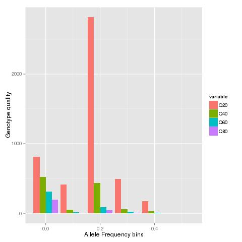
When the VCF file from a published study is run through the script will generate a graph like below:

NOD Mice Substrain Divergence - Runs of Homozygosity

Divergence or rather Differentiation (to use the right terminology), between natural ecotypes or subspecies has been studied in multiple pairs. The broad-scale patterns and underlying processes for such genome wide changes has been studied in detail. 

Do similar processes govern the "divergence" of  artificially inbred strains? Is Drift too strong for background selection to be relevant in such inbred lines? Data [Genetic Analysis of Substrain Divergence in NOD Mice] from a recent study of NOD mice sub-strains might provide some answers. While the study was restricted to sites fixed to homozygosity, it does provide some idea of the major regions that differ between the mouse strains. More detailed analysis of the mouse strains including multiple individuals might be necessary to understand if the diversity landscape of the genome has played any role in shaping the accumulation of genetic differences. 

The Supplementary table 4 provides a list of all the SNP's genotyped using the Mouse Diversity Array. We try to identify runs of homozygosity that share the same genealogy and note if these regions correspond to the deletions identified and validated in the study.

Position				Variants
Chr	Pos (mm10)	Idd.region	SnpId	Type	BomTac	MrkTac	ShiJcl	ShiLtDvs	ShiLt
1	14207005		JAX00242533	G/C	G	G	G	C	C
1	39035554	Idd26	JAX00002691	T/-	T	T	-	T	T
1	39035867	Idd26	JAX00247792	C/-	C	C	-	C	C
1	39035916	Idd26	JAX00002693	A/-	A	A	-	A	A
1	39057575	Idd26	JAX00002694	C/-	C	C	-	C	C
1	111005763	Idd5.4a	JAX00262691	A/-	A	-	A	A	A
1	111014417	Idd5.4a	JAX00262692	T/-	T	-	T	T	T
1	111019979	Idd5.4a	JAX00262694	G/-	G	-	G	G	G
2	83392830		JAX00494876	G/-	-	-	G	-	G
2	131300866	Idd13, Idd13-not B2m	JAX00503778	A/G	A	A	A	G	A
3	8893755		JAX00514596	C/A	C	C	C	C	A
3	24286919		JAX00516977	C/-	C	C	C	-	-
3	24320030		JAX00516979	T/-	T	T	T	-	-
3	24348995		JAX00105316	A/G	A	A	A	-	-
3	24383100		JAX00516985	T/-	T	T	T	-	-
3	33847305		JAX00106024	-/G	G	G	-	G	G
3	33847927		JAX00519037	-/T	T	T	-	T	T
3	33848126		JAX00519038	-/A	A	A	-	A	A
3	33850816		JAX00519044	-/C	C	C	-	C	C
3	33851250		JAX00519045	A/-	A	A	-	A	A
3	33851593		JAX00519046	G/-	G	G	-	G	G
3	65332947		JAX00525208	T/C	T	T	T	T	C
4	44176075		JAX00549396	T/A	T	T	T	A	A
4	95778743		JAX00558533	G/A	G	G	G	A	G
5	22274118		JAX00575925	T/C	T	T	T	T	C
5	41404231		JAX00579937	T/-	T	-	T	T	T
5	66998537		JAX00584961	C/A	C	C	C	C	-
5	73358239		JAX00585757	C/T	C	C	C	T	T
6	38322613		JAX00607572	C/T	C	C	C	C	T
6	53666162		JAX00141075	C/-	T	T	-	T	T
6	61137631		JAX00611572	C/T	C	C	C	T	T
9	7195978		JAX00685032	A/G	A	A	A	G	G
9	29769301		JAX00688769	G/C	G	G	G	G	C
9	106903556		JAX00704737	G/A	G	G	G	G	A
11	3243750		JAX00023793	G/A	G	G	G	A	A
12	39375537		JAX00200149	G/-	G	-	G	G	G
13	116909804	Idd14	JAX00371636	G/A	G	G	G	G	A
15	32687601		JAX00397403	C/A	C	C	C	C	A
15	72708061		JAX00405386	G/A	G	G	G	G	A
16	29905094		JAX00416944	C/-	C	C	-	C	C
16	90657211		JAX00427835	G/A	G	G	G	A	A
18	58558824		JAX00460581	G/T	G	G	G	G	T
18	61847210		JAX00461436	G/A	G	G	G	G	A
18	66105915	Idd21.2	JAX00462793	G/A	G	G	G	A	A
18	84871118	Idd21.1	JAX00467924	-/T	T	T	-	-	-
19	50248464		JAX00479604	C/A	C	C	C	C	A
X	14217495		JAX00177287	C/A	C	C	C	A	A
X	101602508		JAX00716621	G/A	G	G	G	G	A

In the above table the runs of fixed differences and what they are is listed below:

1. First run (marked in blue) of fixed differences corresponds to the Idd26 locus.
2. Next is the Idd5 locus. 
3. The deletion on chromosome 3 spanning 24,272,052 and 24,383,100 has been validated by Sanger sequencing in this study.
4. The second deletion on chromosome 3 spanning as many as 6 SNP's is located rather close to the first deletion.

The remaining clusters of 2 or 3 sites that share the same genealogy are probably too short to correspond to single events themselves. Nonetheless, it would be interesting to see if these fixed differences are localized to lower nucleotide diversity regions in the initial strains.

Bird RNAseq - A thing to watch out for while using the Zebra Finch genome as a reference

Long after our simulation study on RNA-seq, itseems that it is finally time to see some real world use for it. While getting cited many times might suggest some utility for it, being able to actually help real world applications like curing cancer or malaria seems a better reward. 

Downloading a dataset of reads(from a certain bird species) mapped onto the Zebra Finch genome from SRA and calculating the mean mapping quality per gene shows that genes with an Ensemble id greater than ~14,000 have a lower mean mapping quality compared to the rest of the genome. 

This result could potentially be due to the increased mis-mapping seen in our simulation study (see Figure-4). Would discarding multi-mapped reads (zero mapping quality) get rid of this bias? Should this be a issue of major concern? Hopefully, followup studies will appreciate the importance of such bias and try to avoid it or correct for it. 

Ten percent of positively selected variants are within 7 Megabase of the human genome

Ten percent of SNPs that have been found to be positively selected as per the dbPSHP are within a 7 Megabase region on chr 2. This one region is very different from all other regions that have atleast 100 positively selected SNPs in that it has more than 1500 such variants.

1    154500000    167400000    121
10    100100000    113400000    108
12    52200000    62400000    125
14    59800000    70900000    117
15    62900000    79100000    121
17    50350000    64950000    125
18    63400000    67900000    135
2    62400000    75750000    131
2    95500000    101450000    111
2    131100000    137750000    1581
2    175250000    181150000    150
2    194600000    201750000    150
22    28200000    43700000    106
5    9800000    15600000    111
5    106700000    113850000    108
6    25050000    40450000    144
9    97850000    101000000    106
9    122600000    135200000    168

If so many positively selected variants are within such a short distance of each other, can they be considered independent events? Should methods that estimate selection coefficient's consider the cumulative value or just per variant estimates?

Yet another RAD-seq processing tool when genome is available

This is just a simple set of commands to create a RAD-seq processing tool when the genome is available. Since, it accepts reads mapped to genome in a bam file as input, it is capable of handling RAD-seq, exome sequencing as well as low coverage re-sequencing data. Paired-end as well as single end reads are accepted.

 module load samtools  
 module load BEDTools  

 #calculate per site coverage for each individual bam file  
 samtools depth *.sorted.bam > all.coverage  
 #sum the persite coverage across all individuals  
 awk '{for(i=3;i<=NF;i++) t+=$i; print t; t=0}'|sed 's/ /\t/g' all.coverage > persite.coverage  
 #make a histogram of persite coverage across all individuals  
 cut -f 3 persite.coverage |awk '{counts[$1] = counts[$1] + 1; } END { for (val in counts) print val, counts[val]; }'|sort -k1n,1 > persite.coverage.hist  
 #remove sites with more than 200 reads(as inferred from histogram from previous step) per site  
 awk '{for(i=3;i<=NF;i++) t+=$i; if(t<200)print $0; t=0}'|sed 's/ /\t/g' all.coverage > non.repeat.sites  
 #find sites that have atleast 5 reads in 10 individuals  
 awk '{for(i=3;i<=NF;i++) if($i > 5)t++; if(t>10)print $1,$2,$2,t; t=0}' non.repeat.sites|sed 's/ /\t/g' > wellcovered.sites  
 #collapse sites into loci  
 bedtools merge -i wellcovered.sites > wellcovered.sites.bed  
 #call SNP's for selected loci  
 samtools mpileup -l wellcovered.sites.bed -uf ref.fa *.sorted.bam | bcftools view -bvcg - > var.raw.bcf   
 bcftools view var.raw.bcf | vcfutils.pl varFilter -D100 > var.flt.vcf   

Runs of short exons in Titin gene are conserved across all Mammals

Titin gene more commonly known as Connectin is an elastic muscle protein. The complete gene sequence for this gene has been known since 2001. 

Here we compare the exon structure of Titin transcripts across multiple species with special focus on the cluster of short exons(< 100 bp) in the middle of the gene. Exon ranks of these exons is from ~100 to 180.  These exons correspond to the PEVK segments that are thought to provide the protein "spring" like properties. Comparison of the Titin gene across multiple species has previously been performed across large evolutionary distances. 

All four rodent species [Kangaroo rat (Dipodomys ordii), Mouse (Mus musculus), Pika (Ochotona princeps) and Rabbit(Oryctolagus cuniculus)] from Ensembl show the PEVK exons in phase 1 followed by a pair of 3 exons as seen the human titin gene. 

Mouse

Rabbit

Kangroo Rat

Pika

Similarly, all 12 species from Laurasiatheria[Alpaca (Vicugna pacos), Cat (Felis catus),Cow (Bos taurus), Dog (Canis lupus familiaris), Dolphin (Tursiops truncatus), Ferret (Mustela putorius furo), Hedgehog (Erinaceus europaeus), Horse (Equus caballus), Megabat (Pteropus vampyrus), Microbat (Myotis lucifugus), Panda (Ailuropoda melanoleuca), Sheep (Ovis aries)] also have the PEVK cluster.

Alpaca

Cat

Cow

Dog

Dolphin

Ferret

Horse

Megabat

Microbat

Panda

Sheep

The European Hedgehog has only 30 exons annotated in Ensembl release 78. This might change in later releases. So Functional characterization or some other form of validation is required before considering the possibility of the loss of large number of exons.

All 8 primate genomes [Chimpanzee(Pan troglodytes), Gibbon (Nomascus leucogenys), Gorilla (Gorilla gorilla gorilla), Marmoset (Callithrix jacchus), Olive baboon (Papio anubis), Orangutan (Pongo abelii), Tarsier (Tarsius syrichta) and  Vervet-AGM (Chlorocebus sabaeus)] are very similar to the Human titin. The Gibbon TTN gene is not showing the characteristic run of short exons, but this could be due to the Gibbon genome being relatively new.

Gorilla

Chimp

Gibbon

Marmoset

Olive babbon

Tasrsier

Vervet-AGM

Orangutan

While we have looked at birds before, it has not been a complete coverage. Moreover the ortholog for the TTN gene has been named the SPEG complex locus. So here we use the SPEG complex locus transcripts instead of the transcript from the gene annotated as Titin. We can see that the Chinese Turtle (Pelodiscus sinensis) shows the characteristic pattern of the PEVK exons. However, none of the transcripts annotated in birds [falbicollis_ENSFALG00000003453,ggallus_ENSGALG00000028386,acarolinensis_ENSACAG00000013938,mgallopavo_ENSMGAG00000011306 tguttata_ENSTGUG00000006089]

Chinese Turtle

show the pattern.


Another post dealing with Fish, insects and other species might be able to find other interesting changes in the Titin gene during the course of evolution.

Mapping centromeres using Optical Map data

Optical mapping has become rather common for applications ranging from genome assembly improvement and validation to structural variation discovery. Validation of the rice genome using Optical map data also helped map centromeres and even span one centromere. However, in some cases centromeres have been found to correspond to regions that have poor mapping of optical maps, presumably due to the presence of tandem repeats that lack unique restriction sites. Without the availability of genetic linkage maps or other evidence, those working with NGS based draft assemblies have speculated that large gaps in the optical map correspond to centromeres or other repeats.

The Human genome has a higher quality as well as availability of various other resources such as genetic linkage maps, BAC's, FISH etc in addition to the availability of optical mapping data. Centromeres have been mapped in the human genome with various other methods and provides an ideal case to investigate the patterns(or lack thereof) shown by optical maps near centromeres. Optical map data for the human and mouse genome from published studies have been made available as bigBed files. This provides a unique resource to understand the behavior of optical maps near centromeres.

First we download the bigBed files for the human genome Hg38 and convert it to bed12 format. This can then be converted to bed format using the convert perl script

 wget ftp://ngs.sanger.ac.uk/production/grit/track_hub/hg38/om_align_GM10860.bigBed  
 wget ftp://ngs.sanger.ac.uk/production/grit/track_hub/hg38/om_align_GM15510.bigBed  
 wget ftp://ngs.sanger.ac.uk/production/grit/track_hub/hg38/om_align_GM18994.bigBed  
 for i in om_align_GM10860 om_align_GM15510 om_align_GM18994  
 do  
 bigBedToBed "$i".bigBed "$i".bed  
 perl convertBed.pl "$i".bed > "$i"_full.bed  
 done  

Perl script called covertBed.pl to convert bed12 to bed format.

 #!/usr/bin/perl  
 my $bed12file = $ARGV[0];  
 open(FILE1, $bed12file);  
      while($header1=<FILE1>) {  
      chomp $header1;  
      my @parts=split(/\t/,$header1);  
      my @parts2=split(/\,/,$parts[10]);  
      my @parts3=split(/\,/,$parts[11]);  
      my $arrSize = @parts2;  
           for($i=0;$i<$arrSize;$i++){  
           $start=$parts[1]+$parts3[$i];  
           $end=$start+$parts2[$i];  
           print "$parts[0]\t$start\t$end\t$parts2[$i]\n";  
           }  
      }  
 close FILE1;  

We next create 50Kb windows across the human genome to analyze the distribution of cut sites in the Optical map.

 mysql --user=genome --host=genome-mysql.cse.ucsc.edu -B -A -D hg38 -e 'select chrom,size from chromInfo' > chromhg38.genome  
 bedtools makewindows -g chromhg38.genome -w 50000|sort -k1,1 -k2,2n > 50kb.wins  

All 3 Optical maps are combined and the mean of the fragment lengths as well their counts are tabulated in 50Kb windows.

 cat *_full.bed|sort -k1,1 -k2,2n > full_all.bed  
 bedtools map -a 50kb.wins -b full_all.bed -c 4 -o mean -null NA > all.mean  
 bedtools map -a 50kb.wins -b full_all.bed -c 4 -o count -null NA > all.count  

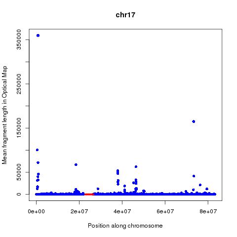
Analysis of these numbers across each chromosome suggests that mean fragment size might be a better predictor of centromeres than the count. The position of the centromeres is obtained from the UCSC tables using below command:

 mysql --user=genome --host=genome-mysql.cse.ucsc.edu -B -A -D hg38 -e 'select chrom,chromStart,chromEnd from centromeres'|grep -v "chromStart" > centromeres.hg38.genome  

Running below R code will create graphical images showing the position of the centromeres by red lines and the mean fragment size by blue dots.

 for (chr in c("chr1","chr2","chr3","chr4","chr5","chr6","chr7","chr8","chr9","chr10","chr11","chr12","chr13","chr14","chr15","chr16","chr17","chr18","chr19","chr20","chr22","chrX"))  
 {  
 read.table(file="all.mean",header=F)->M  
 read.table(file="centromeres.hg38.genome",header=F)->C  
 interleave <- function(v1,v2)  
 {  
 ord1 <- 2*(1:length(v1))-1  
 ord2 <- 2*(1:length(v2))  
 c(v1,v2)[order(c(ord1,ord2))]  
 }  
 jpeg(paste(chr,"_OM.jpeg",sep=""))  
 plot(M$V2[M$V1==chr],M$V4[M$V1==chr],xlab="Position along chromosome",ylab="Mean fragment length in Optical Map",main=chr,col="blue",pch=16)  
 lines(interleave(C$V2[C$V1==chr],C$V3[C$V1==chr]),rep(0.2,length(interleave(C$V2[C$V1==chr],C$V3[C$V1==chr]))),col="red",lwd=5)  
 dev.off()  
 }  

Based on below figures, it can be hypothesized that on chr1, chr2, chr3(to certain extent), chr7, chr9, chr11(to certain extent),chr12,chr13, chr14,chr15 and chr20 the mean optical fragment size goes up near centromeres.

Based on the above analysis can one conclude that it is possible to map Centromeres using Optical mapping data? Far from it, the many false positives and lack of signal in many cases are worrying. The following questions are of importance:

 

1. How does the quality of the genome assembly in the regions adjoining the centromere affect the ability to map centromeres?
2. How does the enzyme used and repeat content and base composition of the centromere affect the precision of attempts aimed at mapping the centromere?