Tuesday, November 25, 2014

Allele frequncies of mutations nearer to genes take time to increase in freequency

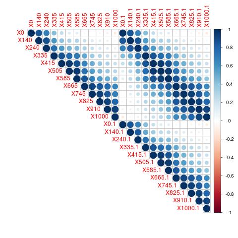
Whole genome sequencing of time course evolving populations is now possible. In their experiment, they monitor the allele frequency of all alleles that reach a frequency greater than 0.1. The fact that the allele frequencies are correlated between time points in both methods used to measure allele frequencies suggests that their method is rather robust. (see correlation plot of allele frequencies at different time points[in minutes]).


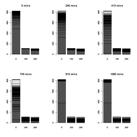
We next explore the change in allele frequency as function of time and distance from the nearest gene. The below plot shows that the allele frequency increases near to genes only in the later stages of the experiment. The first bar represents all the sites nearest to the genes and the bars next to it are those further away from it. Over the time course, the allele frequency of the mutants increase nearer to the gene.


Thursday, November 20, 2014

Novel avian leptin gene is present across the bird phylogeny

Due to the importance of the leptin gene in endocrinology, its existence and behavior in birds have been the focus of considerable debate. The possible inclusion of human contaminant sequences into early bird genome assemblies seems to have been a major complicating factor in understanding Leptin genes in birds. Only recently, with the availability of the Pigeon genome with a well annotated leptin gene has it become evident that birds have a novel gene that has sequence similarity to the mammalian leptin. However, debate regarding its function, tissue specificity and expression patterns are yet to be resolved conclusively. 

With the availability of numerous bird genome assemblies, courtesy of the NGS revolution in sequencing it is now possible to visualize and may be even quantify the prevalence of the leptin gene across different bird groups. Without debating the naming of the leptin like gene annotated in the Pigeon, we take it as given for all our analysis. A simple blastX search provides numerous significant hits. 

Two of the significant hits are from birds, specifically Taeniopygia guttata leptin-like protein precursor and Melopsittacus undulatus leptin precursor. We also get many hits from reptiles before moving to mammals.

Tuesday, November 18, 2014

Optical map dot plot

Using Optical Maps to scaffold genomes of bacteria seems to be a fairly common practice. While it is yet to find widespread use in Eukaryotic species, it has found some success in species such as the cow, rice and parrot.

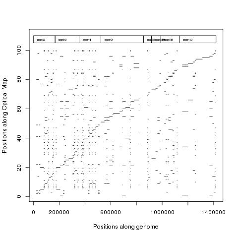
Here we use the assembled Optical map provided as an example with the SOMA package to demonstrate Optical map dot plot creation.

First, we perform an all vs all search between the optical map and in-silico digest of the genome using below script. The script has the parameter called search radius which decides how much flexibility is to be allowed while searching.
 #!/usr/bin/perl   
 use warnings;   
 use Math::Round qw(nearest);  
 use Set::IntSpan;  
 #  
 #perl Map_Optical.pl scaffold.silico soma_format_maps/1.map  
 ## Input parameters  
 %cutlens=();  
 my $roundoffto=10;  
 my $searchradius=200;  
 open CUTSITES, $ARGV[0] or die $!;  
 while($line = <CUTSITES>){  
 chomp $line;  
 my @header = split / /, $line;  
 my $scaffold=$header[0];  
 my $scaflen=$header[1];  
 my $totalcutsites= $header[2];  
 $line = <CUTSITES>;chomp $line;  
 my @cutsites = split / /, $line;  
 my $iso="";  
 my $cutcount=0;  
 my $previous=0;  
   foreach $iso (@cutsites){  
    my $cutlength=$iso-$previous;  
    if($previous>0){  
    $cutcount++;  
    $key=$scaffold . "#" . $cutcount;  
    $cutlens{$cutlength}{$key}=$previous . "_" . $iso;  
    }  
    $previous=$iso;  
    }  
          }#end of while loop  
 close CUTSITES;  
 #print "Done reading Silico-digest provided in file: $ARGV[0]\n";  
 my $mapsite=0;  
 my %mapmaps=();  
 open SOMAP, $ARGV[1] or die $!;   
 while($line = <SOMAP>){   
 chomp $line;  
 my @header2 = split / /, $line;  
 $mapsite++;  
 my $testvalue=$header2[0];  
 my $teststart=$testvalue-$searchradius;  
 my $testend=$testvalue+$searchradius;  
 #print "Searching for $testvalue lengths with a search radius of $searchradius.\n";  
 my $i="";  
 for($i=$teststart;$i<$testend;$i++){  
    foreach my $key (keys %{$cutlens{$i}}) {  
    my @keysp = split /\#/, $key;  
      my @beds= split /\_/, $cutlens{$i}{$key};  
 # scaffold     start     end     map_position     search_radius_hit     map_frag_len     cut_frag_len  
 #   print "$keysp[0]\t$beds[0]\t$mapsite\t$i\t$testvalue\t$keysp[1]\n";  
 #   print "$keysp[0]\t$beds[1]\t$mapsite\t$i\t$testvalue\t$keysp[1]\n";  
 #   print "$keysp[0]\tNA\tNA\n"  
      print "$keysp[0]\t$beds[0]\t$beds[1]\t$mapsite\t$i\t$testvalue\t$keysp[1]\n";  
    }  
 }  
 }#end of while loop  
 close SOMAP;  
After performing a search of the Optical map, the output bed file can be converted into a dotplot file using below script:
 #!/usr/bin/perl  
 use warnings;  
 ##  
 ##perl getfull.pl genome.fa.fai assembled.map.bed   
 ### Input parameters  
 #  
 my %cumlen=();  
 my $cumcount=0;  
 open CUTSITES, $ARGV[0] or die $!;  
 while($line = <CUTSITES>){  
 chomp $line;  
 my @header = split /\t/, $line;  
 $cumlen{$header[0]}=$cumcount;  
 $cumcount=$cumcount+$header[1];  
 }  
 close CUTSITES;  
 open MAPSITES, $ARGV[1] or die $!;  
 while($line = <MAPSITES>){  
 chomp $line;  
 my @header = split /\t/, $line;  
 my $start=$header[1]+$cumlen{$header[0]};  
 my $end=$header[2]+$cumlen{$header[0]};  
 print "Map\t$start\t$header[3]\n";  
 print "Map\t$end\t$header[3]\n";  
 print "Map\tNA\tNA\n";  
 }  
 close MAPSITES;  
The figure below shows the dotplot of the Optical map created using above scripts with a search radius of 200 base pairs. Increasing the search radius saturates the plot while allowing for more distant hits.

Thursday, November 13, 2014

Human chr6 also has the MHC region which shows a DAF peak

Human chr6 has another prominent peak of DAF, corresponding to the MHC region. Flanked by the genes MOG and COL11A2, it spans from approximately 29624758 to 33145670 in the hg19 assembly. Below figure shows the MHC region in blue with the flanking genes in brown. The number of CNV's also jumps up in this region. 


 chr <- "chr6";    
 jpeg(paste("DAF.",chr,".jpeg",sep=""),width=1420)    
 par(mfrow=c(2,1))    
 read.table(file=paste("h.",chr,".mean.bed",sep=""),header=F,stringsAsFactors=F)->M    
 plot(as.numeric(M$V2),as.numeric(M$V4),xlab="Position along chromosome",ylab="Mean derived allele Frequency",main=chr)    
 lines(c(58830166,61830166),c(0.2,0.2),col="red",lwd=5)    
 text(63830166, 0.25,labels="Centromere",col="red")    
 lines(c(171105067,171115067),c(0.3,0.3),col="blue",lwd=5)    
 text(171105067, 0.35,labels="Telomere",col="blue")    
 lines(c(0,10000),c(0.3,0.3),col="blue",lwd=5)    
 text(0, 0.35,labels="Telomere",col="blue")    
 lines(c(57182422,57513376),c(0.25,0.25),col="brown",lwd=5)    
 text(57182422, 0.3,labels="PRIM2 gene",col="brown")    
 M[M$V2>57182422 & M$V3<57513376,]->N   
 points(N$V2,N$V4,pch=13,col="blue")   
 lines(c(33130469,33145670),c(0.35,0.35),col="brown",lwd=5)    
 text(39945670, 0.35,labels="COL11A2 gene",col="brown")    
 lines(c(29624758,29638656),c(0.35,0.35),col="brown",lwd=5)    
 text(25000000, 0.35,labels="MOG gene",col="brown")    
 lines(c(29624758,33145670),c(0.38,0.38),col="blue",lwd=5)    
 text(29624758, 0.42,labels="MHC",col="blue")    
 read.table(file=paste("h.",chr,".countdgv.bed",sep=""),header=FALSE)->C    
 plot(C$V2,C$V4,xlab="Position along chromosome",ylab="Count of known structural variants",main=chr)    
 cor.test(as.numeric(M$V4),C$V4,method="spearman")    
 dev.off()  

Wednesday, November 12, 2014

Human chr6 DAF peak contains PRIM2 gene

Continuing the discussion on DAF's, we look at chr6 and specifically the PRIM2 gene region thought to be under balancing selection.
 chr <- "chr6";   
 jpeg(paste("DAF.",chr,".jpeg",sep=""),width=1420)   
 par(mfrow=c(2,1))   
 read.table(file=paste("h.",chr,".mean.bed",sep=""),header=F,stringsAsFactors=F)->M   
 plot(as.numeric(M$V2),as.numeric(M$V4),xlab="Position along chromosome",ylab="Mean derived allele Frequency",main=chr)   
 lines(c(58830166,61830166),c(0.2,0.2),col="red",lwd=5)   
 text(63830166, 0.25,labels="Centromere",col="red")   
 lines(c(171105067,171115067),c(0.3,0.3),col="blue",lwd=5)   
 text(171105067, 0.35,labels="Telomere",col="blue")   
 lines(c(0,10000),c(0.3,0.3),col="blue",lwd=5)   
 text(0, 0.35,labels="Telomere",col="blue")   
 lines(c(57182422,57513376),c(0.25,0.25),col="brown",lwd=5)   
 text(57182422, 0.3,labels="PRIM2 gene",col="brown")   
 M[M$V2>57182422 & M$V3<57513376,]->N  
 points(N$V2,N$V4,pch=13,col="blue")  
 read.table(file=paste("h.",chr,".countdgv.bed",sep=""),header=FALSE)->C   
 plot(C$V2,C$V4,xlab="Position along chromosome",ylab="Count of known structural variants",main=chr)   
 cor.test(as.numeric(M$V4),C$V4,method="spearman")   
 dev.off()  
The correlation coefficient of 0.2559672 between the mean derived allele frequency and Number of CNV's is line with the results from chr2. The PRIM2 gene that has been shown to have high values of diversity and Tajima's D is located near the centromere and has high mean DAF values. The windows within the PRIM2 gene are marked by blue crosses. 


Monday, November 10, 2014

Human DAF - Derived Allele Frequency plots

A map of recent positive selection in Human genome calculated DAF's apart from various other selection scan statistics. Here we calculate mean DAF's in 50Kb windows for each chromosome and see how it  correlates with CNV density.

Each step and the commands used are documented here:

Use mysql to directly query the UCSC genome browser tables to download the ancestral state of Human SNP's in Chimp, Orangutan and Macaque along with the allele frequencies.

 for i in chr2 chr3 chr4 chr5 chr6 chr7 chr8 chr9 chr10 chr11 chr12 chr13 chr14 chr15 chr16 chr17 chr18 chr19 chr20 chr22 chrX  
 do  
 echo "SELECT t2.chrom,t2.chromStart,t2.chromEnd,t2.name,t2.humanObserved,t2.humanAllele,t2.chimpAllele,t2.orangAllele,t2.macaqueAllele,t1.alleles,t1.alleleFreqs FROM hg19.snp141 AS t1, hg19.snp141OrthoPt4Pa2Rm3 AS t2 WHERE t1.name = t2.name AND t2.chrom='$i'"|mysql --user=genome --host=genome-mysql.cse.ucsc.edu -B -A > human."$i".csv  
 done  

Next, we decide on the ancestral state of each site using parsimony. Sites in which Chimp, Orangutan and Macaque agree are easy to resolve. Similarly, when either the first two (Chimp and Orangutan) or the last two (Orangutan and Macaque) agree, the ancestral state can be decided. In all other cases, we discard the site altogether. Other methods that use Maximum likelihood to infer ancestral state have also been used.
 #!/usr/bin/perl  
 ## Input parameters  
 my $ancfreq = $ARGV[0];  
 open(FILE1, $ancfreq);  
 $header=<FILE1>;#read header  
 while($header=<FILE1>) {  
      $header=~s/\,/\t/g;  
      my @parts=split(/\t/,$header);  
 my $chrom=$parts[0];  
 my $start=$parts[1];  
 my $end=$parts[2];  
 my $chimpA=$parts[6];  
 my $OrgangA=$parts[7];  
 my $MacA=$parts[8];  
 my $anctype= $chimpA. $OrgangA. $MacA;$anctype=~s/(.)(?=.*?\1)//g;  
  if((length $anctype)==1){$found3++;}  
         else{  
             $anctype= $chimpA. $OrgangA;$anctype=~s/(.)(?=.*?\1)//g;  
             if((length $anctype)==1){$foundfirst2++;}  
                 else{  
                 $anctype= $OrgangA. $MacA;$anctype=~s/(.)(?=.*?\1)//g;  
                 if((length $anctype)==1){$foundlast2++;}  
                 elsif((length $anctype)>2){$trial++;$anctype="N";}  
                 else{$anctype="N";$notfound++;}  
                 }  
         }#end of else  
 my $a1=$parts[9];  
 my $a2=$parts[10];  
 my $a1freq=$parts[12];  
 my $a2freq=$parts[13];  
 my $derivedfreq=0;  
 if($anctype=~m/$a2/){$derivedfreq=$a1freq;}  
 elsif($anctype=~m/$a1/){$derivedfreq=$a2freq;}  
 if($derivedfreq>0){print "$chrom\t$start\t$end\t$derivedfreq\t$chimpA\t$OrgangA\t$MacA\t$anctype\n";}  
      }  
 close FILE1;  
 #hg38.snp141OrthoPt4Pa2Rm3.chrom    hg38.snp141OrthoPt4Pa2Rm3.chromStart  hg38.snp141OrthoPt4Pa2Rm3.chromEnd   hg38.snp141OrthoPt4Pa2Rm3.name hg38.snp141OrthoPt4Pa2Rm3.humanObserved hg38.snp141OrthoPt4Pa2Rm3.humanAllele hg38.snp141OrthoPt4Pa2Rm3.chimpAllele  hg38.snp141OrthoPt4Pa2Rm3.orangAllele  hg38.snp141OrthoPt4Pa2Rm3.macaqueAllele hg38.snp141.alleles   hg38.snp141.alleleFreqs  

After deciding on the ancestral state, the derived allele frequency is printed for each of the sites that is retained. The mean DAF can then be easily calculated using the map command in bedtools.

 for i in chr1 chr2 chr3 chr4 chr5 chr6 chr7 chr8 chr9 chr10 chr11 chr12 chr13 chr14 chr15 chr16 chr17 chr18 chr19 chr20 chr21 chr22 chrX  
 do  
 bedtools makewindows -g Homo_sapiens.GRCh37.57.dna.concat.fa.fai -w 50000|awk -v c="$i" '$1==c{print $0}' > "$i".50k.bed  
 perl Afreqbed.pl human."$i".csv > h."$i".bed  
 bedtools map -a "$i".50k.bed -b h."$i".bed -c 4 -o mean > h."$i".mean.bed  
 done  

The mysql interface to UCSC genome browser makes it easy to download all know structural variants from numerous publications.

 mysql --user=genome --host=genome-mysql.cse.ucsc.edu -B -A -e "SELECT * FROM hg19.dgvMerged;" > human_dgvMerged.csv    
Just retaining the co-ordinates (along with length) of the CNV's we create a bed file with below command:

 grep -v "^bin" human_dgvMerged.csv|awk '{print $2,$3,$4,($4-$3)}'|sed 's/ /\t/g' >dgv.bed  

Now that we have everything in the bed format, use the "map" command from bedtools to calculate count of CNV's and plot it for chromosome 2.


 for i in chr1 chr2 chr3 chr4 chr5 chr6 chr7 chr8 chr9 chr10 chr11 chr12 chr13 chr14 chr15 chr16 chr17 chr18 chr19 chr20 chr21 chr22 chrX  
 do  
 bedtools map -a "$i".50k.bed -b dgv.bed -c 3,4 -o count,sum > h."$i".countdgv.bed  
 done  

 chr <- "chr2";  
 jpeg(paste("DAF.",chr,".jpeg",sep=""),width=1420)  
 par(mfrow=c(2,1))  
 read.table(file=paste("h.",chr,".mean.bed",sep=""),header=F,stringsAsFactors=F)->M  
 plot(as.numeric(M$V2),as.numeric(M$V4),xlab="Position along chromosome",ylab="Mean derived allele Frequency",main=chr)  
 lines(c(92326171,95326171),c(0.6,0.6),col="red",lwd=5)  
 text(92326171, 0.65,labels="Centromere",col="red")  
 lines(c(243189373,243199373),c(0.5,0.5),col="blue",lwd=5)  
 text(243189373, 0.55,labels="Telomere",col="blue")  
 lines(c(0,10000),c(0.5,0.5),col="blue",lwd=5)  
 text(0, 0.55,labels="Telomere",col="blue")  
 lines(c(90545103,91545103),c(0.7,0.7),col="green",lwd=5)  
 text(90545103, 0.75,labels="heterochromatin",col="green")  
 lines(c(136545415,136594750),c(0.6,0.6),col="brown",lwd=5)  
 text(136545415, 0.65,labels="LCT gene",col="brown")  
 read.table(file=paste("h.",chr,".countdgv.bed",sep=""),header=FALSE)->C  
 plot(C$V2,C$V4,xlab="Position along chromosome",ylab="Count of known structural variants",main=chr)  
 cor.test(as.numeric(M$V4),C$V4,method="spearman")  
 dev.off()  

We see a positive correlation between mean derived allele frequency and number of known CNV's per 50Kb window with a rho of 0.2496694.
Monday, November 3, 2014

Liftover - what gets lost in translation?

Many genomic analysis require the conversion of genomic coordinates of one genome into another. When a new version of the genome assembly is created, all the data (such as annotation, recombination map, variant calls, genomic features) associated with the older version of the genome need to be "lifted" over to the new genome. 

Similarly, when performing comparative genomic analysis, the homologous regions of genomes need to be identified between genomes that are sometime rather distant. The initial draft annotations of genomes use the lifted over annotations from high quality genomes as the primary raw material. This is an extremely important source of information when RNAseq data is not available. 

Given the increasing importance of such lifting over of genomic coordinates, new tools that can perform this rather simple sounding task are increasing in number. Apart from the established liftOver utility from UCSC, CrossMap, Kraken, NCBI genome remapping service also provide well established pipelines for converting the genomic coordinates for files in different formats such as bed, gff, SAM(& BAM), VCF, Wiggle, BigWig, etc. The UCSC liftOver tool has been implemented in the GALAXY suite, used in VTools, pyliftOver and rtracklayer (a Bioconductor package). All implementations of the UCSC liftover tool as well as CrossMap use the chain files that require many steps to create. If you are lucky enough to be working on one of the genome supported by UCSC, you can download the ready to use chain files directly from the UCSC website.

The original paper that introduced the liftOver utility has some useful technical information about how the the process works and also performance in different regions of the genome. Kraken, uses a different method that does not require all vs all alignments to perform the lifting over of coordinates. One the key features of the liftOver utility is its ability to "handle large gaps" in alignment. Due to its robustness and ease of use, the liftOver utility has been used in numerous studies in very different studies. 

In a series of blog posts, we will analyze and quantify the performance of the UCSC liftOver utility.